CartoDB is a free mapping tool that allows a user to plot place based data on an interactive geographic map (much like a Google map). In CartoDB, you can create static maps or maps in motion, showing how your data moves or changes over time. It also allows you to have multiple layers (up to four in the free edition), which can be turn on and off as well as overlaid on top of each other. CartoDB can be found at: https://cartodb.com. CartoDB and other mapping tools like it are great for providing a visual and geographic representation of data that has a strong sense of place built in. While creating a map will never give the final answer to a research query, maps are helpful in pointing out interesting trends, patterns and connections between different sets of data.
It is easy to sign up for CartoDB (I just used my Google login) and then start creating your map. The easiest way to begin, is to upload a csv file which you can make in any spreadsheet software. This file should contain your data, arranged in columns, with your subject headings across the top. For my example map, I used metadata from the Alabama WPA Slave Narratives provided by Project Guttenberg. My data included columns for the interviewee, interviewer, sex, type of slave (House/Field), when they were interviewed, where they were interviewed, and their place of birth. When importing your data, you can let CartoDB automatically find latitude and longitude coordinates for the place data or you can use the site http://www.mapcoordinates.net/en to manually find the coordinates. (If using the later option, you would need to include a separate column for latitude and a separate column for longitude in your original spreadsheet.)
CartoDB has two different views on the back end (or from the creator’s viewpoint): Data View and Map View. Data view, just as it sounds, looks like a spreadsheet. It allow you to see (and update/correct if necessary) your data. It is also important the CartoDB recognizes the fields with numerical data as a “number” instead of a string of text. (It is easy to change it, by clicking the word “string” under the column heading if needed). Map view actually lets you visually see your data as individual points located on a map.
It is easy to add new layers (by clicking the add feature button on the lower right hand corner and then selecting the data set you would like it to represent). Once you have a layer, you can find it in a tab on the right hand side of the screen. By clicking the paint brush icon, you can change how your data points appear on the map. The default option is “Simple” which basically plots colored dots on your map to correspond with the locations given in your data set. In my example, the Simple map plotted the geographic spot where the interview with the former slave was conducted. Another option is to make a cluster map. In my example, a cluster map showed spots were clusters of interviews were conducted near the same location. The bigger the dot, the more interviews were conducted. You can also change this to a heat map or intensity map, showing more intense colors for bigger groupings instead of bigger dots. Cluster maps can also be animated. Mine showed the locations of interviews over time, using the date and time of the interview as well as the location. This can give you a better idea visually of where interviews were bring conducted concurrently.
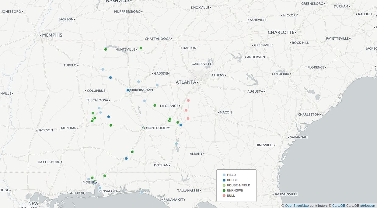
One last type of map I explored was the Category map. This allows you to pick a category of your data and it marks your data points in different colors based on that category. In my example, I picked “Type of Slave” as the category. I end up with a map that still plotted the locations of the interviews, but the dot was light blue if he or she was considered a field slave, dark blue for a house slave, light green for a field and house slave and dark green if the type was unknown. This produced a really interesting map where one could start to draw possible connections between the location the former slave was living when he or she was interviewed and what type of work he or she performed as a slave.
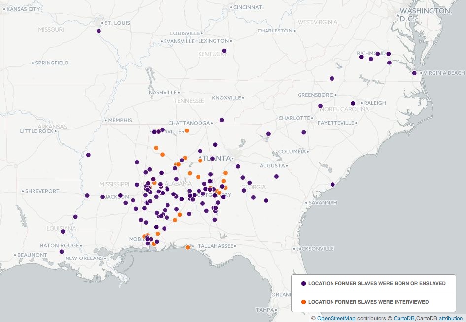
In the end, I included two layers on my sample map: one showing the locations of the interviews and the other showing all the locations the interviewee had lived (as mentioned in the transcript of their interview). This provided a very interesting map, with orange dots (representing the location the former slaves were interviewed) centered in Alabama, and purple dots (representing the locations where former slaves had lived or been born) scattered all over the country from Richmond, VA to a town near Lexington, KY; from Lafayette, LA to St. Louis, MO. This only begins to suggest the large amount of movement that former slaves experienced during their lifetime.